import pandas as pd
from sklearn.model_selection import train_test_split
from sklearn.preprocessing import StandardScaler
from sklearn.compose import ColumnTransformer
from sklearn.feature_extraction.text import TfidfVectorizer
from sklearn.linear_model import Ridge
from sklearn.pipeline import Pipeline
from sklearn.metrics import root_mean_squared_error, mean_absolute_error, r2_score
from sklearn.impute import SimpleImputer

df = pd.read_csv('data/processed_pokemon_cards.csv')4. Transforming, Scaling, and Fitting the Data
Python
Machine Learning
Data Visualization
Loading the Data and Setting Up
Now that we’ve explored our data in part 3, we’re ready to build our predictive model. In this section, we’ll transform and scale our features appropriately, then train a model to predict Pokemon card HP values. Lets start by loading the necessary libraries and our processed dataset.
Preparing the Target Variable
First, we need to separate our target variable (hp) from our features. This is what we’re trying to predict.
target = 'hp'
y = df[target]
Feature Selection
Now we need to prepare our feature set. Based on our exploratory data analysis in part 3, I decided to drop total_resistance_multiplier since it had very little variation and didn’t correlate well with HP. We also need to handle any missing text values by filling them with empty strings.
cols_to_drop = ['hp', 'total_resistance_multiplier']
X = df.drop(columns=cols_to_drop)

X['flavorText'] = X['flavorText'].fillna("")
X['ability_text'] = X['ability_text'].fillna("")
Categorizing Features by Type
Different types of features need different preprocessing steps. Lets organize our features into three categories: numeric features (need scaling), text features (need TF-IDF vectorization), and binary features (can be used as-is).
numeric_features = [
    'level', 'convertedRetreatCost', 'number', 'primary_pokedex_number',
    'pokemon_count', 'total_weakness_multiplier', 'total_weakness_modifier',
    'total_resistance_modifier', 'pokedex_frequency', 'artist_frequency',
    'ability_count', 'attack_count', 'max_damage', 'attack_cost'
]

text_features = ['flavorText', 'ability_text']

binary_features = [
    col for col in X.columns if col not in numeric_features and col not in text_features
]

print(f"Numeric features: {len(numeric_features)}")
print(f"Text features: {len(text_features)}")
print(f"Binary features: {len(binary_features)}")
Numeric features: 14
Text features: 2
Binary features: 93We can see that we have 14 numeric features, 2 text features, and many binary features (mostly from our one-hot encoding in part 2).
Train-Test Split
Before we do any transformations, we need to split our data into training and testing sets. This ensures we don’t leak information from the test set into our model. I’m using a 50/50 split to have enough data for both training and testing.
X_train, X_test, y_train, y_test = train_test_split(X, y, test_size=0.5, random_state=123)Building the Preprocessing Pipeline
Now comes the important part - setting up our preprocessing pipeline. We need to:
- Numeric features: Impute missing values with the median, then standardize (scale to mean=0, std=1)
- Binary features: Pass through unchanged since they’re already in the right format
- Text features: Convert to TF-IDF vectors with a maximum of 100 features each
We’ll use scikit-learn’s ColumnTransformer to apply different preprocessing steps to different feature types, and then combine everything with a Ridge regression model in a single pipeline.
numeric_pipeline = Pipeline(steps=[
    ('impute', SimpleImputer(strategy='median')),
    ('scale', StandardScaler())
])

preprocessor = ColumnTransformer(
    transformers=[
        ('numeric', numeric_pipeline, numeric_features),

        ('pass', 'passthrough', binary_features),

        ('tfidf_flavor',
            TfidfVectorizer(stop_words='english', max_features=100),
            'flavorText'),

        ('tfidf_ability',
            TfidfVectorizer(stop_words='english', max_features=100),
            'ability_text')
    ],
    remainder='drop'
)

model_pipeline = Pipeline(steps=[
    ('preprocessor', preprocessor),
    ('model', Ridge(alpha=1.0))
])

model_pipeline.fit(X_train, y_train)
y_pred = model_pipeline.predict(X_test)
The pipeline automatically handles all the preprocessing steps and then trains our Ridge regression model. I chose Ridge regression because it adds L2 regularization, which helps prevent overfitting by penalizing large coefficients.
Evaluating Model Performance
Now lets see how well our model performs on the test set. We’ll look at several metrics to understand different aspects of model performance.
rmse = root_mean_squared_error(y_test, y_pred)
print(f"RMSE: {rmse:.2f} hp")

X_train_transformed = preprocessor.fit_transform(X_train)
print(f"Shape of transformed training data: {X_train_transformed.shape}")

mae = mean_absolute_error(y_test, y_pred)
print(f"MAE: {mae:.2f} hp")

r2 = r2_score(y_test, y_pred)
print(f"R-Squared: {r2:.3f}")
RMSE: 15.22 hp
Shape of transformed training data: (2235, 307)
MAE: 11.22 hp
R-Squared: 0.939These metrics tell us:
- RMSE (Root Mean Squared Error): The average prediction error in HP units. Lower is better.
- MAE (Mean Absolute Error): Similar to RMSE but less sensitive to outliers. Also in HP units.
- R-Squared: The proportion of variance explained by the model. Values closer to 1.0 indicate better fit.
Visualizing Predictions
Lets create a scatter plot to visualize how well our predictions match the actual HP values. Points closer to the red diagonal line indicate better predictions.
import matplotlib.pyplot as plt
import seaborn as sns

plt.figure(figsize=(8, 8))
sns.scatterplot(x=y_test, y=y_pred)
plt.xlabel("Actual HP (y_test)")
plt.ylabel("Predicted HP (y_pred)")
plt.title("Actual vs. Predicted HP")

# Add the "perfect prediction" line
plt.plot([y_test.min(), y_test.max()], [y_test.min(), y_test.max()], 'r--', lw=2)
plt.show()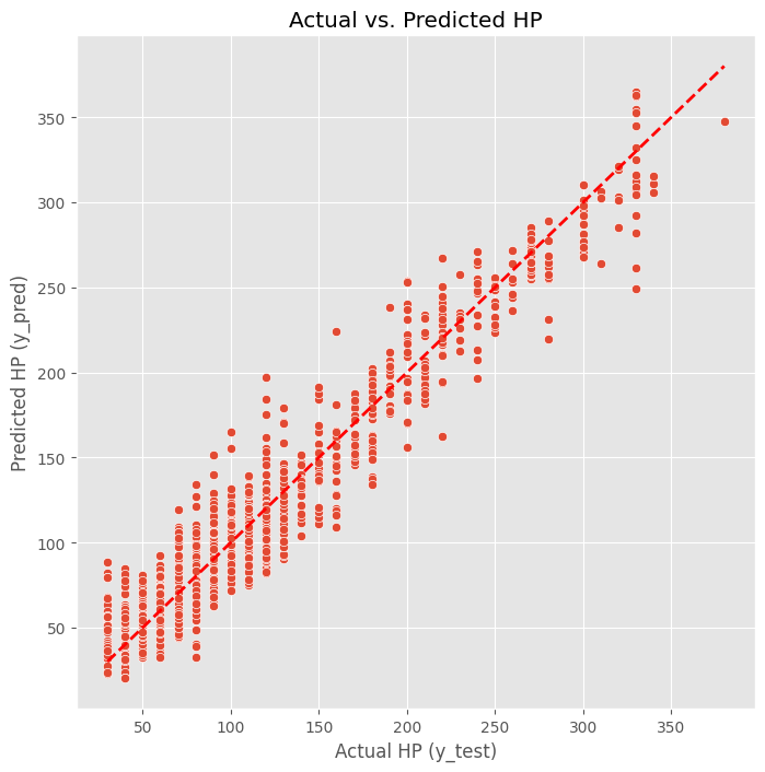
From this plot, we can see how the predictions compare to actual values. If the model were perfect, all points would fall on the red line. The spread around the line shows us where the model is making errors.
Feature Importance Analysis
One of the advantages of using Ridge regression is that we can examine the coefficients to understand which features are most important for predicting HP. Lets extract and analyze these coefficients.
model = model_pipeline.named_steps['model']

preprocessor = model_pipeline.named_steps['preprocessor']

numeric_features = preprocessor.transformers_[0][2]
binary_features = preprocessor.transformers_[1][2]

tfidf_flavor_names = preprocessor.named_transformers_['tfidf_flavor'].get_feature_names_out()
tfidf_ability_names = preprocessor.named_transformers_['tfidf_ability'].get_feature_names_out()

all_feature_names = \
    list(numeric_features) + \
    list(binary_features) + \
    list(tfidf_flavor_names) + \
    list(tfidf_ability_names)

coefficients = pd.Series(model.coef_, index=all_feature_names)

print("--- Most Positive Features (increase HP) ---")
print(coefficients.sort_values(ascending=False).head(10))

print("\n--- Most Negative Features (decrease HP) ---")
print(coefficients.sort_values(ascending=True).head(10))

print("\n--- Features Closest to Zero (least important) ---")
print(coefficients.abs().sort_values().head(10))
--- Most Positive Features (increase HP) ---
subtype_VMAX 116.304684
subtype_V-UNION 68.144272
subtype_V 67.655707
rarity_Special Illustration Rare 52.443085
rarity_Ultra Rare 52.268106
subtype_TAG TEAM 50.894390
subtype_EX 49.716326
rarity_Double Rare 47.923288
subtype_GX 47.201676
subtype_ex 43.102486
dtype: float64
--- Most Negative Features (decrease HP) ---
subtype_Basic -54.956849
subtype_Restored -49.572918
ex -46.475835
subtype_Stage 1 -31.499100
rarity_Rare Holo EX -30.052394
rarity_Rare Shining -30.022542
type_Metal -28.546938
dark -28.255926
subtype_Prism Star -24.088233
rarity_Rare Prism Star -24.088233
dtype: float64
--- Features Closest to Zero (least important) ---
rarity_Rare Holo LV.X 0.000000
subtype_Level-Up 0.000000
has_pokemon_power 0.000000
has_ancient_trait 0.000000
attacking 0.020297
attach 0.069256
level 0.091615
water 0.110130
poisoned 0.137334
cause 0.148945
dtype: float64Interpreting the Results
The feature importance analysis shows us:
- Most Positive Features: These features are associated with higher HP values. When these features increase, the predicted HP tends to increase.
- Most Negative Features: These features are associated with lower HP values. They might represent basic or early-evolution Pokemon that typically have less HP.
- Features Near Zero: These features have little impact on HP predictions and could potentially be removed in future iterations.
This analysis helps us understand what the model learned about Pokemon cards and validates whether its findings align with our domain knowledge about the Pokemon card game.
Next Steps
Now that we have a working model, there are several ways we could improve it:
- Try different models (Random Forest, Gradient Boosting, etc.)
- Tune hyperparameters more carefully
- Engineer additional features based on our findings
- Address any outliers or problematic data points
- Investigate why certain predictions are far from actual values
This baseline model gives us a solid foundation to build upon and helps us understand which features matter most for predicting Pokemon card HP.